Why this article

The more I have to interact with customers asking about MySQL/Galera, the most I have to answer over and over to the same question about what kind of network conditions Galera can manage efficiently.

One of the most frequent myths I have to cover at the start of any conversation that involve the network is PING.

Most of the customers use PING to validate the generic network conditions, and as direct consequence they apply that approach also when in need to have information on more complex and heavy use like in the Galera replication.

To have a better understanding why I consider the use of PING, not wrong but inefficient, let us review some basic networking concepts.

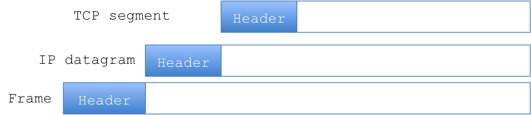
Frame

At the beginning stay the physical layer, but I am going to skip it otherwise article will be too long, what I want only to say is that unless you are able to afford a leased line to connect to your distributed sites, you are going to be subject to Packet switching, as such affected by: throughput, bandwidth, latency, congestion, and dropped packets issues.

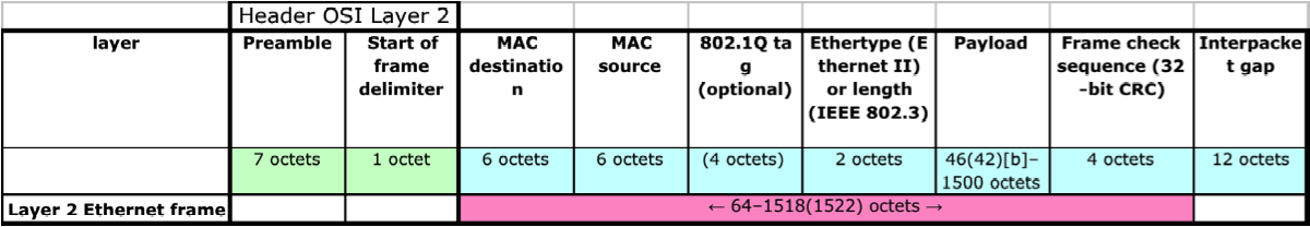
Given the physical layer, and given we are talking about Ethernet connections, the basic transporter and the vector that encapsulates all the others is the Ethernet frame. A frame can have a dimension up to 1518 bytes and nothing less then 64.

A frame has a header compose by:

• Preamble of 7 bytes,
• Delimiter 1 bytes,
• MAC address destination 6 bytes,
• MAC address destination 6 bytes,
• Optional fields (IEEE 802.1Q/ IEEE 802.1p), 4 bytes
• Ethernet type or length (if > 1500 it represent the type; if < 1501 it represents the length of the Payload, 2 bytes
• PayLoad, up to 1500 bytes
• Frame CRC, 4 bytes
• Inter-packet gab, this is the space that is added between to frames

A frame can encapsulate many different protocols like:

• IPv4
• IPv6
• ARP
• AppleTalk
• IPX
• ... Many more

The maximum size available for the datagram to be transmitted is of 1500 bytes, also known as MTU. That is, the MTU or Maximum transmission unit is the dimension in bytes that a frame can transport from source to destination, we will see after that this is not guarantee and fragmentations can happen.

Only exception is when Jumbo Frames are supported, in that case a frame can support a payload with a size up to 9000 bytes. Jumbo frames can be quite bad for latency, especially when the transmission is done between data-centre geographically distributed.

IP (internet protocol)

For the sake of this article we will focus on the IPv4 only. The IPv4 (Internet Protocol) is base on the connectionless and best-effort packets delivery, this means that each frame is sent independently, the data is split in N IP datagram and sent out to the destination, no guarantee it will deliver or that the frames will arrive in the same order they are sent.

Each IP datagram has a header section and data section.

The IPv4 packet header consists of 14 fields, of which 13 are required.

The 14th field is optional (red background in table) and aptly named: options.

An IP datagram is encapsulated in the frame…

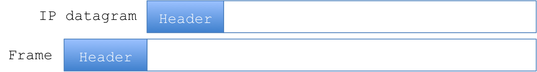
Then sent.

For performance the larger is the datagram (1500 MTU), the better, but this only in theory, because this rules works fine when a datagram is sent over a local network, or a network that can guarantee to keep the level of MTU to 1500.

What happen in real life is that a frame sent over the Internet has to go over many different networks and there is no guarantee that all of them will support the same MTU, actually the normal condition is that they don’t.

So when a frame pass trough a gateway, the gateway knows the MTU of the two links (in/out) and if they do not match, it will process the frame fragmenting it.

See below:

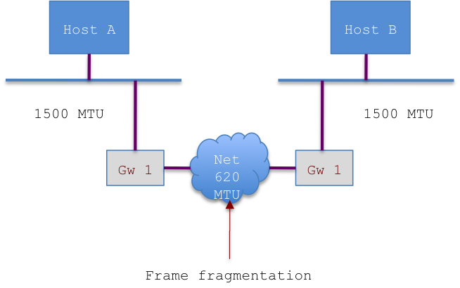
Assuming Host A is sending an IP datagram of 1400 bytes to Host B, when Gw1 will receive it, it will have to fragment it in to smaller peaces to allow the frame to be transported:

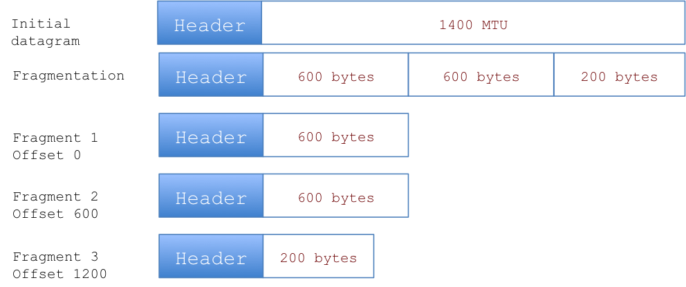
Once a datagram is fragmented to match the largest transportable frame, it will be recompose only at destination. If one of the fragments of the datagram is lost, for any reason, the whole datagram got discarded and transmission fails.

ICMP

The IP specification imposes the implementation of a special protocol dedicated to the IP status check and diagnostics, the ICMP (Internet Control Message Protocol).

Any communication done by ICMP is embedded inside an IP datagram, and as such follow the same rules:

ICMP has many “tools” in his pocketknife, one if them is PING.

A ping is compose by a echo request datagram and an echo reply datagram:

Request and reply have a similar definition, with the note that the replay MUST contain the full set of data sent by the echo request.

Ping by default sent a set of data of 56 bytes plus the bytes for the ICMP header, so 64 bytes.

Ping can be adjust and to behave in different way, including the data dimension and the don’t fragment bit (DF). The last one is quite important because this set the bit that will mark the datagram as not available for fragmentation.

As such if you set a large dimension for the data and set the DF, the datagram will be sent requesting to not be fragmented, in that case if a frame will reach a gateway that will require the fragmentation the whole datagram will be drop, and we will get an error.

I.e.:

ping -M do -s 1472 -c 3 192.168.0.34
 PING 192.168.0.34 (192.168.0.34) 1472(1500) bytes of data.
 1480 bytes from 192.168.0.34: icmp_req=1 ttl=128 time=0.909 ms
 1480 bytes from 192.168.0.34: icmp_req=2 ttl=128 time=0.873 ms
 1480 bytes from 192.168.0.34: icmp_req=3 ttl=128 time=1.59 ms

as you can see I CAN send it using my home wireless because is below 1500 MTU also if I ask to do not fragment, this because my wireless is using 1500MTU.

But if I just raise the dimension of ONE byte:

ping -M do -s 1473 -c 3 192.168.0.34
 PING 192.168.0.34 (192.168.0.34) 1473(1501) bytes of data.
 From 192.168.0.35 icmp_seq=1 Frag needed and DF set (mtu = 1500)
 From 192.168.0.35 icmp_seq=1 Frag needed and DF set (mtu = 1500)
 From 192.168.0.35 icmp_seq=1 Frag needed and DF set (mtu = 1500)

Removing the –M (such that fragmentation can take place)

root@tusacentral01:~# ping  -s 1473 -c 3 192.168.0.34

PING 192.168.0.34 (192.168.0.34) 1473(1501) bytes of data.
 1481 bytes from 192.168.0.34: icmp_req=1 ttl=128 time=1.20 ms
 1481 bytes from 192.168.0.34: icmp_req=2 ttl=128 time=1.02 ms
 1481 bytes from 192.168.0.34: icmp_req=3 ttl=128 time=0.996 ms

PING is widely used to test connectivity between two network points, which is good, and from the example above, you may think that it is a good tool to test the network also in more complex situations, like when we need to be sure that the virtually synchronous galera replication will NOT be affected.

But you are wrong, the PING tool as part of the ICPM for his operations it is still using the basic IP protocol which is base on the best effort delivery of the datagram, while any data that is transmitted between the nodes in a MySQL/Galera cluster, use the TCP protocol, the two are bound (from TCP point of view), but the TCP implementation behaviour is quite different.

To understand that let us review at very high level (one billion of kilometres high) the TCP characteristics.

TCP

As mentioned previously the IP and related ICPM work on the base of the best effort delivery of the datagram, what this means in short is that whatever I sent using it is sent without guarantee it will reach destination, and without actually caring to send it if it fails, more no real check is perform between source and destination regarding the data transmission.

TCP means Transmission Control Protocol and as the name says, it is design to control the data transmission happening between source and destination.

TCP’s implementations offer a reliable, ordered, error-checked delivery of a stream of octets between source and destination.

The TCP is a transmission protocol and as such it works at the transport level of the OSI model:

TCP implementations use the IP protocol encapsulation for the transmission of the data:

A TCP implementation has several characteristics that make sense to summarize:

• Is stream oriented, that' it when two applications open a connection base on TCP, they will see it as a stream of bit that will be deliver to the destination application, exactly in the same order and consistency they had on the source.
• Establish a connection, which means that the host1 and host2 before start to send data over, must perform a handshake operation, which will allow them to know each other state. Connection use a three way handshake:

Once it is establish the two parts will keep to monitor the data transfer, in case of crash interruption of the service both hosts will notify the application involved in the stream transfer.

• TCP sees a connection
• Buffered transmission, the applications communicating the data can choose whatever dimension to send, it could be a single byte a time. The transport layer will buffer the data in order to match the best datagram dimension for that specific moment, and will send it. The dimension of the datagram is adaptative which means it can be adjusted in relation to the network transfer condition.
• Unstructured stream, meaning the stream does not have a predefine format/dimension for internal data, as such the applications must know how to read from the stream.
• Full-duplex connection, data can be transmitted simultaneously from both side.
• Segment TCP implementation see the stream as a sequence of octet (bytes), which it will split in segments, the segment dimension is normally as large as a datagram.

TCP header definition:

Source port (16 bits)

As said TCP implementations are reliable and can re-transmit missed packets, let see how it works:

This mechanism is in place for each TCP transmission, and ensures the correct send/receive of the segment.

It is easy to understand how also if effective, having this mechanism working for a single segment at time is far to be efficient.  This because considering a set of packages from 1 to 100, before sending package 2, the dispatch of package 1 must be acknowledge.

To solve this issue, the TCP use the concept of dynamic slide window. That’s it the TCP implementations manage to dispatch multiple packages at the same time:

A sliding window in TCP implementations works at octet level not by segment or by package, each stream’s octet has a sequential number, the dispatcher manages three pointers associated to each connection.

The first pointer indicate the start of the sliding window, splitting the octet that had be dispatched & acknowledge from the ones that are in progress or still to dispatch.

The second pointer indicates the higher octet that can be dispatch before getting the acknowledgments for the already dispatched octet.

The third pointer indicates the window limit after which no dispatch can be done, until further slide.

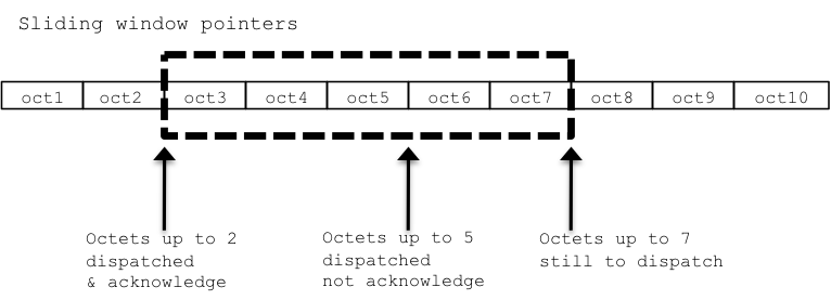
In TCP implementation the slide window has, as previously mentioned, a dynamic dimension, each acknowledgement received is also containing a declaration of how many octet the receiver can accept.

The whole discussion now will become much more complex and not pertinent to the scope of this article, but is worth to mention that, it is here that the whole concept of flow/congestion control will take place.

For the sake of this article and simplifying a lot let us say that when there are optimal conditions in a local lan the dimension of a segment will coincide with the maximum MTU available.

While when sending traffic over the internet, the TCP implementation will have to manage not only the optimal initial dimension, but possible and probable issue while the transmission will take place, reducing and enlarging the sliding window as needed, and in some cases put it on hold.

If you are really interested on how congestion works in the TCP/IP world I suggest this book (http://www.amazon.com/Adaptive-Congestion-Networks-Automation-Engineering-ebook/dp/B008NF05DQ)

Back to the topic

So we have seen how PING works, and the fact it send a simple echo request, using a very basic datagram, with no dispatch or connection error handling.

On the other hand we have see how complex TCP implementation is, and how important is in the TCP implementation the concept of adaptative transmission (that will also seriously affected by available bandwidth) and congestion control.

Keeping that in mind, there is no way we can compare a TCP/IP data transmission between to points with a simple ICMP/IP echo, no matter how large we will make the datagram, or if we declare it not to fragment, or whatever a Ping is executing and following a different protocol, and should never be used to validate the data transmission in a TCP/IP scenario.

Back to square 1, how I can evaluate my connection between two geographically distributed sites?  In detail how I can be sure the transfer will be efficient enough to support the Galera replication?

When implementing Galera, some additional status metrics are added in MySQL, two of them are quite relevant to the purpose of this article:

• Wsrep replicated bytes
• Wsrep received bytes

If you are smart, and I am sure you are, you already have some historical monitor in place, and before even thinking to go for geographical distributed replication you have tested and implement MySQL/Galera using local cluster.

As such you will have collected data about the two metrics above, and will be easy to identify the MAX value, be careful here do not use the average.

Why? Because the whole exercise is to see if the network can efficiently manage the traffic of a (virtually) synchronous connection, without having the Galera flow control to take place.

As such let us say we have 150Kb/s as replicated bytes, and 300k as received, and see what will happen if we use PING and another tool more TCP oriented.

In the following scenario I am going to first check if the two locations are connected using a high-speed link that will allow 1500 MTU, then I will check the connection state/latency using the max dimension of 300K.

 Test 1

[root@Machine1~]# ping -M  do -s 1432 -c 3 10.5.31.10

PING 10.5.31.10 (10.5.31.10) 1432(1460) bytes of data.

From 192.168.10.30 icmp_seq=1 Frag needed and DF set (mtu = 1398)

From 192.168.10.30 icmp_seq=2 Frag needed and DF set (mtu = 1398)

From 192.168.10.30 icmp_seq=2 Frag needed and DF set (mtu = 1398)

 Test 2

[root@Machine1~]# ping -M  do -s 1371 -c 3 10.5.31.10

PING 10.5.31.10 (10.5.31.10) 1371(1399) bytes of data.

From 192.168.10.30 icmp_seq=1 Frag needed and DF set (mtu = 1398)

From 192.168.10.30 icmp_seq=1 Frag needed and DF set (mtu = 1398)

From 192.168.10.30 icmp_seq=1 Frag needed and DF set (mtu = 1398)

Test 3

[root@Machine1~]# ping -M  do -s 1370 -c 3 10.5.31.10

PING 10.5.31.10 (10.5.31.10) 1370(1398) bytes of data.

1378 bytes from 10.5.31.10: icmp_seq=1 ttl=63 time=50.4 ms

1378 bytes from 10.5.31.10: icmp_seq=2 ttl=63 time=47.5 ms

1378 bytes from 10.5.31.10: icmp_seq=3 ttl=63 time=48.8 ms

As you can see the link is not so bad, it can support 1370 MTU, so in theory we should be able to have a decent connection.

Let see... what happens with PING

[root@Machine1~]# ping   -c 3 10.5.31.10

PING 10.5.31.10 (10.5.31.10) 56(84) bytes of data.

64 bytes from 10.5.31.10: icmp_seq=1 ttl=63 time=49.6 ms

64 bytes from 10.5.31.10: icmp_seq=2 ttl=63 time=46.1 ms

64 bytes from 10.5.31.10: icmp_seq=3 ttl=63 time=49.7 ms

--- 10.5.31.10 ping statistics ---

3 packets transmitted, 3 received, 0% packet loss, time 2052ms

rtt min/avg/max/mdev = 46.189/48.523/49.733/1.650 ms

[root@Machine1~]# ping -M  do -s 300 -c 3 10.5.31.10

PING 10.5.31.10 (10.5.31.10) 300(328) bytes of data.

308 bytes from 10.5.31.10: icmp_seq=1 ttl=63 time=50.5 ms

308 bytes from 10.5.31.10: icmp_seq=2 ttl=63 time=48.5 ms

308 bytes from 10.5.31.10: icmp_seq=3 ttl=63 time=49.6 ms

--- 10.5.31.10 ping statistics ---

3 packets transmitted, 3 received, 0% packet loss, time 2053ms

rtt min/avg/max/mdev = 48.509/49.600/50.598/0.855 ms

Performing the tests seems that we have more ore less 49-50 ms latency, which is not really great, but manageable, we can play a little with flow-control in Galera and have the sites communicating, with that I am NOT recommending to set a Galera cluster with 50ms latency, what I am saying is that if desperate something can be done, period.

But wait a minute let us do the other test, and this time let us use a tool that is design for checking the real condition of a network connection using TCP/IP.

For that I normally use NetPerf (there are other tools, but I like this one).

About NetPerf:

"Netperf is a benchmark that can be used to measure the performance of many different types of networking. It provides tests for both unidirectional throughput, and end-to-end latency. The environments currently measureable by netperf include:

TCP and UDP via BSD Sockets for both IPv4 and IPv6

DLPI

Unix Domain Sockets

SCTP for both IPv4 and IPv6"

(http://www.netperf.org/netperf/)

NetPerf use a two-point connection instantiating a server demon on one machine, and using an application that simulate the client-server scenario.

I strongly suggest you to read the documentation, to better understand what it can do, how and the results.

Done? Ready let us go...

Given NetPerf allow me to define what is the dimension I need to send, and what I will receive, this time I can set the test properly, and ask what will be the real effort:

[root@Machine1~]# netperf -H 10.5.31.10 -t TCP_RR -v 2 -- -b 6 -r 156K,300k

MIGRATED TCP REQUEST/RESPONSE TEST from 0.0.0.0 (0.0.0.0) port 0 AF_INET to 10.5.31.10 () port 0 AF_INET : first burst 6

Local /Remote

Socket Size   Request  Resp.   Elapsed  Trans.

Send   Recv   Size     Size    Time     Rate

bytes  Bytes  bytes    bytes   secs.    per sec

65536  87380  159744   300000  10.00      30.20

65536  87380

Alignment      Offset         RoundTrip  Trans    Throughput

Local  Remote  Local  Remote  Latency    Rate     10^6bits/s

Send   Recv    Send   Recv    usec/Tran  per sec  Outbound   Inbound

8         0          0        0       231800.259 30.198   38.592     72.476

The tool will use a TCP round trip, as such it will simulate a real TCP connection/stream/sliding-window/traffic-congestion-control.

The result is 231800.259 microseconds for latency; also other metrics are interesting but for consistency with ping let us stay on latency.

So we have 231800.259 microseconds that mean 231.8 millisecond, real latency.

This result is quite different from the PING results, reason for that is as said a totally different transport mechanism, which will imply a different cost.

Considering the number of 231.8 ms a site-to-site synchronous replication is out of the question.

I can then focus and spend my time to explore different and more appropriate solutions.

Conclusion(s)

The conclusion(s) is quite simple, whenever you need to validate your network connection PING is fine.

Whenever you need to measure the capacity of your network, then PING is just dangerous, and you should really avoid using it.

Good MySQL to all.