"What happens when you run a 10 TB MySQL database on Kubernetes?"
That's the question many of our customers and users asked and honestly, we were extremely curious ourselves. 
So, we ditched the weekend plans, rolled up our sleeves, and jumped down the rabbit hole. What we found was far more challenging (and perhaps a bit more "psychedelic") than expected. We spent days rigorously testing the Percona Operator for PXC at massive scale.
This blog post distills all our findings into the most critical, actionable advice you need to ensure your high-scale environment not only survives but operates reliably.
If you are lazy and prefer to watch a video, here is the presentation I did at the MySQL Belgian days in January 2026.
First of all, what environment did we use?
Well forget about 4Gb ram or using the millesimal set on CPUs. You need heavy stuff, you need power, you need the mega-super-duper tank not the small bike, well if you can pay for it of course. Anyhow we have tested on something that is not small and not too huge as well, all in AWS/EKS.
The AWS instance type chosen for the testing environment was m7i.16xlarge, combined with an io2 storage class provisioned at 80,000 IOPS.
This configuration was selected because:
- The m7i.16xlarge is a general-purpose instance with custom 4th Generation Intel Xeon Scalable processors, offering 64 vCPUs and 256 GiB of high-bandwidth DDR5 memory. This robust computational and memory capacity ensures that CPU or memory are unlikely to be limiting factors during initial testing of a large-scale, high-performance MySQL cluster on EKS.
- Its 20 Gbps dedicated EBS bandwidth and up to 80,000 maximum IOPS to EBS perfectly complement the high-performance io2 Block Express storage volume.
- By provisioning the storage to the maximum rated IOPS of the underlying instance type, the aim was to create a stress-testing environment that isolates potential performance constraints in the MySQL operator, Percona architecture, Kubernetes storage mechanisms (CSI/EBS), or database configuration, rather than hitting a hardware-imposed ceiling. This allows for a precise analysis of operational overheads and bottlenecks when the I/O subsystem is not the weakest link, which is critical when scaling a database to 10 TB of data.
Did it go as we would like to? Well long story short, not in full but I was expecting worse … into the rabbit hole we go.

We fully validated the cluster's ability to scale, but here's what surprised (and alarmed) us the most:
- The 16-Hour Naptime MTTR (Mean Time To Recover): Full cluster recovery time for the 10 TB dataset clocked in at an eye-watering 960 minutes (16 hours)! If your business requires a guaranteed 1-hour Recovery Time Objective (RTO), you're going to have a very awkward conversation with your boss.
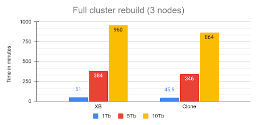
The rebuild operation from cluster crash was executed recovering the first node from snapshot then, letting the cluster recover using internal recovery mechanism.
- The Unruly Cloud Storage: We provisioned high-performance AWS EBS volumes (80,000 IOPS), yet we hit a wall due to Galera Flow Control. The root cause? One node's volume had a 21% performance degradation compared to the others. The entire synchronous cluster was choked by the single slowest volume.
- The Starved Recovery Container: We discovered the restore process's most time-consuming phase the single-threaded redolog apply was bottlenecked because the default recovery container only gets a laughably default memory allocation (around 100 MB). This process consumed 92% of the total restore time.
The Safe Operation Playbook: Critical Fixes
You can tame the data monster, but you have to stop using the default settings. Your focus must shift to I/O consistency, recovery optimization, and mandatory zero-downtime practices.
1. Stop Starving Your Recovery Container
The single most effective action to improve your RTO is giving the restore container more memory to efficiently process the redolog.
- The Fix: You must override the inadequate defaults in your recovery.yaml specification.
- Recommendation: Set memory: 4Gi and cpu: 2000m (2 full cores). This directly reduces the time spent on the single-threaded redolog apply phase, chipping away at that painful 16-hour recovery window. This will alleviate and not resolve the situation though.
- Redefine Recovery SLO: Since the Operator waits for full cluster recovery before HAProxy serves traffic, you must redefine your internal service goal to Minimal High Availability (HA) (two out of three nodes synced), you can achieve it increasing the size of the cluster by steps, so first one node then add the second and so on. This allows you to claim service is resumed in hours (or less, if optimized) rather than 16 hours.
2. The Cloud Storage Problem: EBS is Not Trustable
For critical, high-scale PXC clusters, the testing proved that high-cost abstracted cloud volumes (EBS) are too unpredictable due to the risk of I/O variability.
- The Problem: I/O variance is a single point of failure that triggers Galera Flow Control. Because PXC is synchronous, if one node is 21% slower, the entire cluster is 21% slower.
- The Long-Term Solution: For mission-critical 10 TB systems, mandate a review for dedicated storage solutions. Look for cloud alternatives that offer strict I/O guarantees, such as dedicated NVMe instances, to bypass the performance abstraction layer and ensure every node performs equally. Or opt for direct attach (fiberchannel) solutions with a SAN tune to prevent volume overlaps.
3. Zero-Downtime is Mandatory (Say No to Direct SQL DDL)
On a Percona XtraDB Cluster, DDL is replicated using Total Order Isolation (TOI). This means that direct ALTER TABLE operations cause a full, unacceptable table lock, resulting in downtime.
- The Rule: Use PTOSC (Percona Online Schema Change) for all DDL, including simple index operations. It takes significantly longer, but it is the only way to avoid service interruption.
- The Capacity Warning: PTOSC temporarily duplicates the entire target table. Ensure you have meticulous capacity planning for temporary disk space to prevent a cluster-wide storage saturation crash!
- Large DML: Break all large UPDATE and DELETE operations into small, iterative batches (chunks) to minimize the scope and duration of transactional locks.
Hot Data Subset vs. The Whole Barn
The most fascinating performance finding was how much the application's access pattern affects performance at scale. This dictates how well your InnoDB Buffer Pool can save you from a slow disk.
| Access Pattern | Description | Performance Outcome |
| Skewed/Live Subset (Pareto) | Application uses a small, "hot" subset of data (e.g., the last few weeks' transactions). | Good. The Buffer Pool works perfectly. We saw lower I/O Wait (IOWAIT) and sustained high throughput up to 4024 concurrent threads. The 10 TB cluster runs like a 1 TB cluster. |
| Uniform Access | Queries are distributed uniformly across the entire dataset (10 TB). | Not so good. Forces high disk activity because the Buffer Pool cannot cache everything. Resulted in high IOWAIT and immediate performance degradation past the CPU limit. |
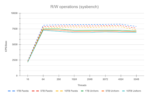
Remember that the tests used a 50/50 read/write workload. Even when operating on a "hot" subset in the buffer pool, the persistent write and purge operations still required disk I/O, which likely reduced the visible performance difference (delta) between the hot subset and uniform access patterns. This delta would be larger with a higher percentage of read operations.
The Bottom Line is that your 10 TB cluster is faster if your application keeps queries focused on the "hot" data subset. Uniform access patterns force the system to pay the full 10 TB I/O cost, every time.
Actionable Summary for the Team
- Recovery Override: Set memory: 4Gi in the recovery spec to reduce the negative impact of the 92% redolog apply bottleneck.
- DDL Enforcement: PTOSC is mandatory for all schema changes. Batch large DML.
- Storage Fix: Do not trust EBS/abstracted storage for 10 TB. Plan an architectural shift toward guaranteed I/O (e.g., dedicated NVMe instances).
- Data Mobility: Standardize on MyDumper/Loader for all bulk operations.
- Data distribution/access: If You Have a Hot Data Subset, Offload the Rest. The better performance seen with the "hot" data subset (Pareto) is your green light!
Any data your application accesses uniformly (or rarely) is only increasing your recovery time and operational cost.
You should treat the remaining data as a candidate for immediate migration to an OLAP container or data lake, ensuring your PXC cluster remains lean and fast.
Conclusions
Ultimately, our deep dive proved that running Percona XtraDB Cluster on Kubernetes with a 10 TB dataset is less about raw scalability and more about operational rigor and resource tuning.
The cluster is fundamentally resilient, but its success hinges on bypassing the hidden pitfalls like:
- the unpredictable nature of abstract cloud I/O
- the crippling cost of default recovery settings
- the unacceptable downtime from standard DDL practices.
However we also identify some areas for improvements like in the case of full cluster recovery, we will work on that.
The key takeaway is simple: default configurations are for small data, large datasets require deliberate engineering.
Notes:
* In this context means: Mean Time To Recover / Restore (The "User" Metric). Which is the average time from the start of the outage until the system is fully back online and usable for the customer. Includes: Detection time + Response time + Repair time + Testing time.